Gradient descent and beyond

In machine learning, optimization is king. Finding the best possible values for a model's parameters is crucial for creating accurate models that can yield useful predictions. At the heart of a machine learning algorithm lies a powerful optimization technique known as gradient descent that iteratively tweaks a model's parameters in the direction of steepest descent, minimizing its loss function. Beyond this foundational method lies a wealth of extensions, refinements, and alternatives developed over the years to tackle the challenges of modern machine learning. In this article, I'll briefly introduce the Gradient Descent and Newton method techniques in their simplest form. Stay tuned for more articles on this topic.

Vanilla gradient descent

Gradient descent is an algorithm that minimizes a given model's loss function based on calculating the gradients of the loss landscape. Believe it or not, Gradient Descent was introduced by mathemetician and physicist Louis Augustin Cauchy in 1847.

We start with a loss/error function that qunatifies the distance between a model's predictions and the true values. Starting out with random weights, the goal is to tweak them until the error is as small as possible.

Tweaking the parameters is done by calculating the gradient of the loss function at a specific point and determining which direction we need to take to minimize the loss. This is given by

where is the learning rate or step size.

Gradient

The gradient is a vector of first-order derivatives of a scalar-valued function. It is given by:

The gradient helps us measure the direction of the fastest rate of increase; but in GD, we negate this expression because we're interested in the fastest rate of descent. Imagine looking down at the peak of a mountain range; what is the quickest path to the bottom? That is what the gradient tells us for any function in .

Let's begin with a simple example. How do you find the minimum of the following function?

Let's first calculate the gradient of w.r.t , which is simply the derivative:

Then let's set the learning rate and pick a random point , to begin with. We can then take steps in the direction of the negative gradient of the function as follows, using the gradient descent equation we defined above:

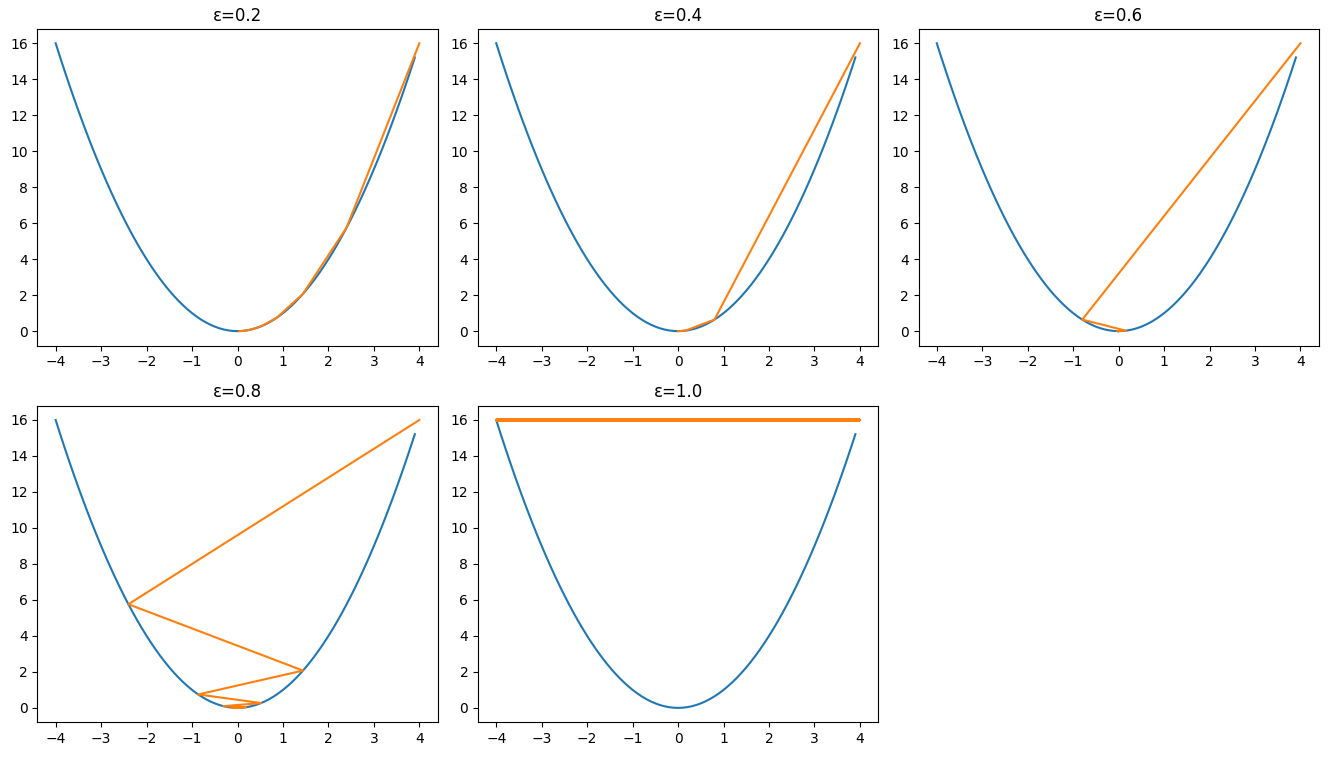
As we can see in the figures above, picking a suitable value for is very important to ensure that our algorithm behaves correctly. Selecting a value for that is too small can result in us undershooting the minimum and taking a long time to arrive there ( figure). On the other hand, if we pick a value for that is too large, we risk overshooting the minimum, as shown in the figure.

And that's it (for the simplest form of GD)! We calculated the gradient of , defined our optimization method , picked a suitable value for our learning rate , selected a random starting point and successfully found the minimum.

In practice, we are often interested in finding the minimum of much more complicated functions over many iterations, known as forward and backward propagation, but that's a topic for another time.

Bonus: why stop at the gradient?

Newton's method and the Hessian

Newton's method is another powerful optimization technique that can help us minimize our loss function . Unlike Gradient Descent, Newton's method requires that our loss function be twice-differentiable.

The Hessian matrix is a matrix of the second derivatives of a multivariate function. It describes the curvature of the landscape produced by that function. In other words, the Hessian matrix tells us how much the gradient of a function changes as we move along each coordinate axis.

We define the Hessian matrix of a function as follows:

Here, is the Hessian matrix of the function evaluated at point , and is its -th entry.

Also, note that if the second derivatives are continuous, the differential operators are commutative,

Taylor Approximation

Because the Hessian matrix requires an enormous amount of compute and is sometimes intractable, we look to approximate it using a second-order Taylor approximation around the current point :

Here, is the gradient of the function evaluated at point . And this approximation is helpful because it captures the local behavior of the function around the point .

Recall that an update is given by,

Therefore, the new point is given by . If we substitute this expression in the approximation, we get,

where, is the original value of the funciton, is the expected imporvement due to the function's slope, and is the correction to account for the function's curvature.

Note that when is large enough, the algorithm can diverge. On the other hand, if our approximation is sufficiently accurate, we converge very quickly.

Finally, the different terms in the Taylor approximation are just tools to help us adjust to the different properties of the landsacape. If the last term is positive, the optimal step that effectively decreases the Taylor approximation yields:

We can use this optimal step size to update our current point as follows:

This update rule is known as the Newton-Raphson method, and it can converge much faster than gradient descent since it takes into account the curvature of the landscape. However, the computation of the Hessian matrix can be expensive for high-dimensional functions, and it may not always be positive definite, which is a requirement for the method to work properly.

In practice, gradient descent is often a more practical optimization algorithm, as it is simpler to implement and can work well for many optimization problems. However, there are cases where Newton-Raphson method or its variants, such as quasi-Newton methods like Broyden-Fletcher-Goldfarb-Shanno (BFGS) and limited-memory BFGS (L-BFGS), can outperform gradient descent.

And just like that, we have successfully defined two of the most important optimzation methods in modern optimization theory. If you found this useful and would like to be notified of future articles on (but not limited to) the following topics:

• Computation theory
• ML
• System design
• Miscellaneous

Drop your email here